Plotting
This page describes in depth the general plotting capabilities of GCPy, including possible argument values for every plotting function.
For information about GCPy functions that are specific to the GEOS-Chem benchmark workflow, please see our Benchmarking chapter.
Six-panel comparison plots
The functions listed below generate six-panel plots comparing variables between two datasets:
Plotting function |
Located in module |
|---|---|
|
|
|
Both compare_single_level() and compare_zonal_mean()
generate a six panel plot for each variable passed. These plots can
either be saved to PDFs or generated sequentially for visualization in
the Matplotlib GUI using matplotlib.pyplot.show().
Each plot uses data passed from a reference (Ref) dataset
and a development (Dev) dataset. Both functions share
significant structural overlap both in output appearance and code
implementation.
You can import these routines into your code with these statements:
from gcpy.plot.compare_single_level import compare_single_level
from gcpy.plot.compare_zonal_mean import compare_zonal_mean
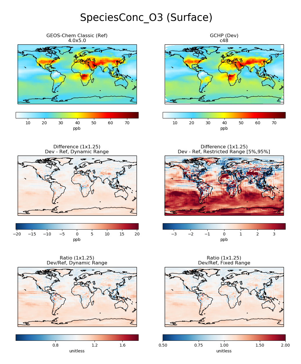
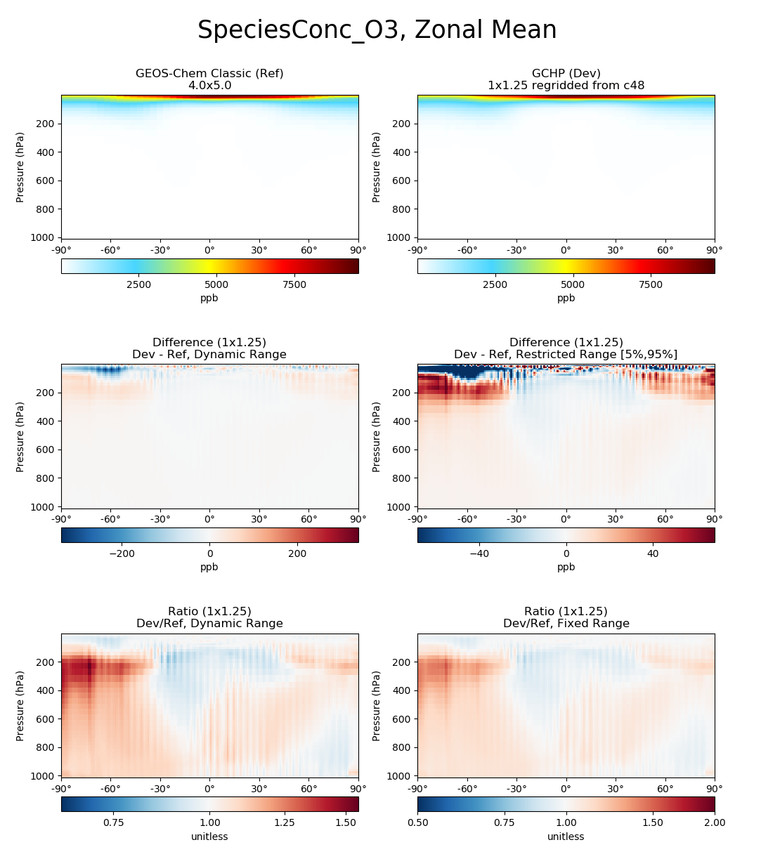
Each panel has a title describing the type of panel, a colorbar for
the values plotted in that panel, and the units of the data plotted in
that panel. The upper two panels of each plot show actual values from
the Ref (left) and Dev (right) datasets for a
given variable. The middle two panels show the difference
(Dev - Ref) between the values in the Dev
dataset and the values in the Ref dataset. The left middle
panel uses a full dynamic color map, while the right middle panel caps
the color map at the 5th and 95th percentiles. The bottom two panels
show the ratio (Dev/Ref) between the values in the Dev
dataset and the values in the Ref Dataset. The left bottom panel uses
a full dynamic color map, while the right bottom panel caps the color
map at 0.5 and 2.0.
Function compare_single_level
The compare_single_level function accepts takes the following
arguments:
def compare_single_level(
        refdata,
        refstr,
        devdata,
        devstr,
        varlist=None,
        ilev=0,
        itime=0,
        refmet=None,
        devmet=None,
        weightsdir='.',
        pdfname="",
        cmpres=None,
        match_cbar=True,
        normalize_by_area=False,
        enforce_units=True,
        convert_to_ugm3=False,
        flip_ref=False,
        flip_dev=False,
        use_cmap_RdBu=False,
        verbose=False,
        log_color_scale=False,
        extra_title_txt=None,
        extent=None,
        n_job=-1,
        sigdiff_list=None,
        second_ref=None,
        second_dev=None,
        spcdb_files=None,
        ll_plot_func='imshow',
        **extra_plot_args
):
    """
    Create single-level 3x2 comparison map plots for variables common
    in two xarray Datasets. Optionally save to PDF.

    Args:
        refdata: xarray dataset
            Dataset used as reference in comparison
        refstr: str
            String description for reference data to be used in plots
        devdata: xarray dataset
            Dataset used as development in comparison
        devstr: str
            String description for development data to be used in plots

    Keyword Args (optional):
        varlist: list of strings
            List of xarray dataset variable names to make plots for
            Default value: None (will compare all common variables)
        ilev: integer
            Dataset level dimension index using 0-based system.
            Indexing is ambiguous when plotting differing vertical grids
            Default value: 0
        itime: integer
            Dataset time dimension index using 0-based system
            Default value: 0
        refmet: xarray dataset
            Dataset containing ref meteorology
            Default value: None
        devmet: xarray dataset
            Dataset containing dev meteorology
            Default value: None
        weightsdir: str
            Directory path for storing regridding weights
            Default value: None (will create/store weights in
            current directory)
        pdfname: str
            File path to save plots as PDF
            Default value: Empty string (will not create PDF)
        cmpres: str
            String description of grid resolution at which
            to compare datasets
            Default value: None (will compare at highest resolution
            of ref and dev)
        match_cbar: bool
            Set this flag to True if you wish to use the same colorbar
            bounds for the Ref and Dev plots.
            Default value: True
        normalize_by_area: bool
            Set this flag to True if you wish to normalize the Ref
            and Dev raw data by grid area. Input ref and dev datasets
            must include AREA variable in m2 if normalizing by area.
            Default value: False
        enforce_units: bool
            Set this flag to True to force an error if Ref and Dev
            variables have different units.
            Default value: True
        convert_to_ugm3: bool
            Whether to convert data units to ug/m3 for plotting.
            Default value: False
        spcdb_files: str | list
            A single species_database.yml file or a list of files
            (e.g. for Ref & Dev).  Only used when convert_ugm3=True.
            Default value: None
        flip_ref: bool
            Set this flag to True to flip the vertical dimension of
            3D variables in the Ref dataset.
            Default value: False
        flip_dev: bool
            Set this flag to True to flip the vertical dimension of
            3D variables in the Dev dataset.
            Default value: False
        use_cmap_RdBu: bool
            Set this flag to True to use a blue-white-red colormap
            for plotting the raw data in both the Ref and Dev datasets.
            Default value: False
        verbose: bool
            Set this flag to True to enable informative printout.
            Default value: False
        log_color_scale: bool
            Set this flag to True to plot data (not diffs)
            on a log color scale.
            Default value: False
        extra_title_txt: str
            Specifies extra text (e.g. a date string such as "Jan2016")
            for the top-of-plot title.
            Default value: None
        extent: list
            Defines the extent of the region to be plotted in form
            [minlon, maxlon, minlat, maxlat].
            Default value plots extent of input grids.
            Default value: [-1000, -1000, -1000, -1000]
        n_job: int
            Defines the number of simultaneous workers for parallel
            plotting.  Set to 1 to disable parallel plotting.
            Value of -1 allows the application to decide.
            Default value: -1
        sigdiff_list: list of str
            Returns a list of all quantities having significant
            differences (where |max(fractional difference)| > 0.1).
            Default value: None
        second_ref: xarray Dataset
            A dataset of the same model type / grid as refdata,
            to be used in diff-of-diffs plotting.
            Default value: None
        second_dev: xarray Dataset
            A dataset of the same model type / grid as devdata,
            to be used in diff-of-diffs plotting.
            Default value: None
        ll_plot_func: str
            Function to use for lat/lon single level plotting with
            possible values 'imshow' and 'pcolormesh'. imshow is much
            faster but is slightly displaced when plotting from
            dateline to dateline and/or pole to pole.
            Default value: 'imshow'
        extra_plot_args: various
            Any extra keyword arguments are passed through the
            plotting functions to be used in calls to pcolormesh() (CS)
            or imshow() (Lat/Lon).
    """
and generates a comparison plot such as:
Function compare_zonal_mean
def compare_zonal_mean(
        refdata,
        refstr,
        devdata,
        devstr,
        varlist=None,
        itime=0,
        refmet=None,
        devmet=None,
        weightsdir='.',
        pdfname="",
        cmpres=None,
        match_cbar=True,
        pres_range=None,
        normalize_by_area=False,
        enforce_units=True,
        convert_to_ugm3=False,
        spcdb_files=None,
        flip_ref=False,
        flip_dev=False,
        use_cmap_RdBu=False,
        verbose=False,
        log_color_scale=False,
        log_yaxis=False,
        extra_title_txt=None,
        n_job=-1,
        sigdiff_list=None,
        second_ref=None,
        second_dev=None,
        ref_vert_params=None,
        dev_vert_params=None,
        **extra_plot_args
):
    """
    Creates 3x2 comparison zonal-mean plots for variables
    common in two xarray Datasets. Optionally save to PDF.

    Args:
        refdata: xarray dataset
            Dataset used as reference in comparison
        refstr: str
            String description for reference data to be used in plots
        devdata: xarray dataset
            Dataset used as development in comparison
        devstr: str
            String description for development data to be used in plots

    Keyword Args (optional):
        varlist: list of strings
            List of xarray dataset variable names to make plots for
            Default value: None (will compare all common 3D variables)
        itime: integer
            Dataset time dimension index using 0-based system
            Default value: 0
        refmet: xarray dataset
            Dataset containing ref meteorology
            Default value: None
        devmet: xarray dataset
            Dataset containing dev meteorology
            Default value: None
        weightsdir: str
            Directory path for storing regridding weights
            Default value: None (will create/store weights in
            current directory)
        pdfname: str
            File path to save plots as PDF
            Default value: Empty string (will not create PDF)
        cmpres: str
            String description of grid resolution at which
            to compare datasets
            Default value: None (will compare at highest resolution
            of Ref and Dev)
        match_cbar: bool
            Set this flag to True to use same the colorbar bounds
            for both Ref and Dev plots.
            Default value: True
        pres_range: list of two integers
            Pressure range of levels to plot [hPa]. The vertical axis
            will span the outer pressure edges of levels that contain
            pres_range endpoints.
            Default value: [0, 2000]
        normalize_by_area: bool
            Set this flag to True to to normalize raw data in both
            Ref and Dev datasets by grid area. Input ref and dev
            datasets must include AREA variable in m2 if normalizing
            by area.
            Default value: False
        enforce_units: bool
            Set this flag to True force an error if the variables in
            the Ref and Dev datasets have different units.
            Default value: True
        convert_to_ugm3: str
            Whether to convert data units to ug/m3 for plotting.
            Default value: False
        spcdb_files: str | list
            A single species_database.yml file or a list of files
            (e.g. for Ref & Dev).  Only used when convert_to_ugm3=True.
            Default value: None
        flip_ref: bool
            Set this flag to True to flip the vertical dimension of
            3D variables in the Ref dataset.
            Default value: False
        flip_dev: bool
            Set this flag to True to flip the vertical dimension of
            3D variables in the Dev dataset.
            Default value: False
        use_cmap_RdBu: bool
            Set this flag to True to use a blue-white-red colormap for
            plotting raw reference and development datasets.
            Default value: False
        verbose: logical
            Set this flag to True to enable informative printout.
            Default value: False
        log_color_scale: bool
            Set this flag to True to enable plotting data (not diffs)
            on a log color scale.
            Default value: False
        log_yaxis: bool
            Set this flag to True if you wish to create zonal mean
            plots with a log-pressure Y-axis.
            Default value: False
        extra_title_txt: str
            Specifies extra text (e.g. a date string such as "Jan2016")
            for the top-of-plot title.
            Default value: None
        n_job: int
            Defines the number of simultaneous workers for parallel
            plotting.  Set to 1 to disable parallel plotting.
            Value of -1 allows the application to decide.
            Default value: -1
        sigdiff_list: list of str
            Returns a list of all quantities having significant
            differences (where |max(fractional difference)| > 0.1).
            Default value: None
        second_ref: xarray Dataset
            A dataset of the same model type / grid as refdata,
            to be used in diff-of-diffs plotting.
            Default value: None
        second_dev: xarray Dataset
            A dataset of the same model type / grid as devdata,
            to be used in diff-of-diffs plotting.
            Default value: None
        ref_vert_params: list(AP, BP) of list-like types
            Hybrid grid parameter A in hPa and B (unitless).
            Needed if ref grid is not 47 or 72 levels.
            Default value: None
        dev_vert_params: list(AP, BP) of list-like types
            Hybrid grid parameter A in hPa and B (unitless).
            Needed if dev grid is not 47 or 72 levels.
            Default value: None
        extra_plot_args: various
            Any extra keyword arguments are passed through the
            plotting functions to be used in calls to pcolormesh()
            (CS) or imshow() (Lat/Lon).
    """
and generates a comparison plot such as:
Example script
Here is a basic script that calls both compare_zonal_mean() and
compare_single_level():
#!/usr/bin/env python

import xarray as xr
import matplotlib.pyplot as plt
from gcpy.plot.compare_single_level import compare_single_level
from gcpy.plot.compare_zonal_mean import compare_zonal_mean

file1 = '/path/to/ref'
file2 = '/path/to/dev'
ds1 = xr.open_dataset(file1)
ds2 = xr.open_dataset(file2)
compare_zonal_mean(ds1, 'Ref run', ds2, 'Dev run')
plt.show()
compare_single_level(ds1, 'Ref run', ds2, 'Dev run')
plt.show()
Single panel plots
Function single_panel() (contained in GCPy module
gcpy.plot.single_panel) is used to create plots containing
only one panel of GEOS-Chem data. This function is used within
compare_single_level() and compare_zonal_mean() to
generate each panel plot. It can also be called directly on its
own to quickly plot GEOS-Chem data in zonal mean or single level
format.
Function: single_panel
Function single_panel() accepts the following arguments:
def single_panel(
        plot_vals,
        ax=None,
        plot_type="single_level",
        grid=None,
        gridtype="",
        title="fill",
        comap=WhGrYlRd,
        norm=None,
        unit="",
        extent=None,
        masked_data=None,
        use_cmap_RdBu=False,
        log_color_scale=False,
        add_cb=True,
        pres_range=None,
        pedge=np.full((1, 1), -1),
        pedge_ind=np.full((1, 1), -1),
        log_yaxis=False,
        xtick_positions=None,
        xticklabels=None,
        proj=ccrs.PlateCarree(),
        sg_path='',
        ll_plot_func="imshow",
        vert_params=None,
        pdfname="",
        weightsdir='.',
        vmin=None,
        vmax=None,
        return_list_of_plots=False,
        **extra_plot_args
):
    """
    Core plotting routine -- creates a single plot panel.

    Args:
        plot_vals: xarray.DataArray, numpy.ndarray, or dask.array.Array
            Single data variable GEOS-Chem output to plot

    Keyword Args (Optional):
        ax: matplotlib axes
            Axes object to plot information
            Default value: None (Will create a new axes)
        plot_type: str
            Either "single_level" or "zonal_mean"
            Default value: "single_level"
        grid: dict
            Dictionary mapping plot_vals to plottable coordinates
            Default value: {} (will attempt to read grid from plot_vals)
        gridtype: str
            "ll" for lat/lon or "cs" for cubed-sphere
            Default value: "" (will automatically determine from grid)
        title: str
            Title to put at top of plot
            Default value: "fill" (will use name attribute of plot_vals
            if available)
        comap: matplotlib Colormap
            Colormap for plotting data values
            Default value: WhGrYlRd
        norm: list
            List with range [0..1] normalizing color range for matplotlib
            methods. Default value: None (will determine from plot_vals)
        unit: str
            Units of plotted data
            Default value: "" (will use units attribute of plot_vals
            if available)
        extent: tuple (minlon, maxlon, minlat, maxlat)
            Describes minimum and maximum latitude and longitude of input
            data.  Default value: None (Will use full extent of plot_vals
            if plot is single level).
        masked_data: numpy array
            Masked area for avoiding near-dateline cubed-sphere plotting
            issues  Default value: None (will attempt to determine from
            plot_vals)
        use_cmap_RdBu: bool
            Set this flag to True to use a blue-white-red colormap
            Default value: False
        log_color_scale: bool
            Set this flag to True to use a log-scale colormap
            Default value: False
        add_cb: bool
            Set this flag to True to add a colorbar to the plot
            Default value: True
        pres_range: list(int)
            Range from minimum to maximum pressure for zonal mean
            plotting. Default value: [0, 2000] (will plot entire
            atmosphere)
        pedge: numpy array
            Edge pressures of vertical grid cells in plot_vals
            for zonal mean plotting.  Default value: np.full((1, 1), -1)
            (will determine automatically)
        pedge_ind: numpy array
            Index of edge pressure values within pressure range in
            plot_vals for zonal mean plotting.
            Default value: np.full((1, 1), -1) (will determine
            automatically)
        log_yaxis: bool
            Set this flag to True to enable log scaling of pressure in
            zonal mean plots.  Default value: False
        xtick_positions: list(float)
            Locations of lat/lon or lon ticks on plot
            Default value: None (will place automatically for
            zonal mean plots)
        xticklabels: list(str)
            Labels for lat/lon ticks
            Default value: None (will determine automatically from
            xtick_positions)
        proj: cartopy projection
            Projection for plotting data
            Default value: ccrs.PlateCarree()
        sg_path: str
            Path to NetCDF file containing stretched-grid info
            (in attributes) for plot_vals.
            Default value: '' (will not be read in)
        ll_plot_func: str
            Function to use for lat/lon single level plotting with
            possible values 'imshow' and 'pcolormesh'. imshow is much
            faster but is slightly displaced when plotting from dateline
            to dateline and/or pole to pole.  Default value: 'imshow'
        vert_params: list(AP, BP) of list-like types
            Hybrid grid parameter A in hPa and B (unitless). Needed if
            grid is not 47 or 72 levels.  Default value: None
        pdfname: str
            File path to save plots as PDF
            Default value: "" (will not create PDF)
        weightsdir: str
            Directory path for storing regridding weights
            Default value: "." (will store regridding files in
            current directory)
        vmin: float
            minimum for colorbars
            Default value: None (will use plot value minimum)
        vmax: float
            maximum for colorbars
            Default value: None (will use plot value maximum)
        return_list_of_plots: bool
            Return plots as a list. This is helpful if you are using
            a cubedsphere grid and would like access to all 6 plots
            Default value: False
        extra_plot_args: various
            Any extra keyword arguments are passed to calls to
            pcolormesh() (CS) or imshow() (Lat/Lon).

    Returns:
        plot: matplotlib plot
            Plot object created from input
    """
Function single_panel() expects data with a 1-length (or
non-existent) T (time) dimension, as well as a
1-length or non-existent Z (vertical level) dimension.
single_panel() contains a few amenities to help with plotting
GEOS-Chem data, including automatic grid detection for lat/lon or
standard cubed-sphere xarray DataArray-s. You can also pass NumPy
arrays to plot, though you’ll need to manually pass grid info in this
case (with the gridtype, pedge, and
pedge_ind keyword arguments).
The sample script shown below shows how you can data at a single level and
timestep from an xarray.DataArray object.
#!/usr/bin/env python

import xarray as xr
import matplotlib.pyplot as plt
from gcpy.plot.single_panel import single_panel

# Read data from a file into an xr.Dataset object
dset = xr.open_dataset('GEOSChem.SpeciesConc.20160701_0000z.nc4')

# Extract ozone (v/v) from the xr.Dataset object,
# for time=0 (aka first timestep) and lev=0 (aka surface)
sfc_o3 = dset['SpeciesConcVV_O3'].isel(time=0).isel(lev=0)

# Plot the data!
single_panel(sfc_o3)
plt.show()