Plotting output from code profilers
GCPy contains functions to plot output from the gprofng and Intel VTune code profilers, which can help you to identify computational bottlenecks (aka “hotspots”) in GEOS-Chem Classic, GCHP, and HEMCO.
gprofng
This example demonstrates how you can plot function profiles generated by the gprofng performance profiler.
Source code
Description |
Script location |
|---|---|
Usage
First, generate a function profile with gprofng:
$ gprofng collect app /path/to/executable/file
where /path/to/executable/file is the path to the program that
you wish to profile. For example, to profile GEOS-Chem Classic, you
would use this command:
$ gprofng collect app ./gcclassic
Gprofng will send profiling output to a folder named
test.N.er, where N is an integer index and er
stands for “experiment record”.
Next, send function profiling information to a file:
$ echo functions | gprofng display text test.N.er > functions_profile.txt
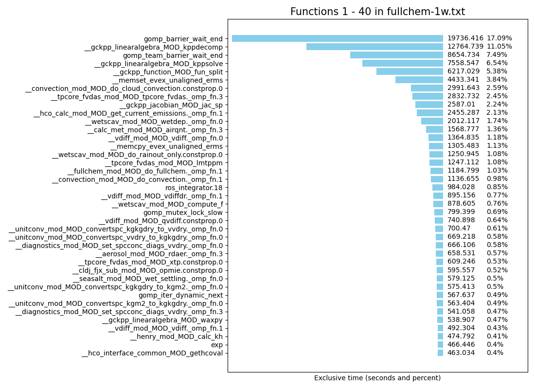
Here is a sample functions_profile.txt for GEOS-Chem Classic.
(gp-display-text) Functions sorted by metric: Exclusive Total CPU Time

Excl. Total     Incl. Total      Name
CPU             CPU
   sec.      %     sec.      %
508.406 100.00  508.406 100.00   <Total>
 62.594  12.31   62.594  12.31   __unitconv_mod_MOD_convertbox_kgm2_to_kg
 61.653  12.13   61.653  12.13   __unitconv_mod_MOD_convertbox_kg_to_kgm2
 58.401  11.49   58.401  11.49   <static>@0x7696c (<libm-2.28.so>)
 46.833   9.21   64.075  12.60   __tomas_mod_MOD_mnfix
 41.609   8.18   41.609   8.18   __gckpp_linearalgebra_MOD_kppdecomp
 29.941   5.89   29.941   5.89   __gckpp_linearalgebra_MOD_kppsolve
 26.609   5.23   26.609   5.23   __gckpp_function_MOD_fun_split
 ... etc ...
The Excl. Total (total Exclusive Time) metric is useful for identifying computational bottlenecks. This represents the amount of time spent in a subroutine, excluding time spent in any subroutines called by the subroutine.
Make sure that you have specified the proper Matplotlib backend for your system. Also activate your GCPy Python environment with:
$ conda activate gcpy_env
Then run the example script with the following command:
(gcpy_env) $ python -m gcpy.profile.gprofng_functions functions_profile.txt 1 40
This will create a plot similar to that shown above, which shows the top 40 functions sorted by exclusive time. To see the next 40 functions sorted by exclusive time, use this command:
(gcpy_env) $ python -m gcpy.profile.gprofng_functions functions_profile.txt 41 80
etc. You should display fewer than 50 functions in order to prevent the time and percent labels from overlapping.
You may now deactivate the Python environment.
$ conda deactivate
Intel VTune
These examples demonstrate how you can display output from the Intel VTune profiler in an easy-to-read format.
Source code
Description |
Script location |
|---|---|
Usage
First, use Intel VTune to collect information about hotspots:
$ vtune -collect hotspots -- /path/to/executable/file
where /path/to/executable/file is the path to the program that
you wish to profile. For example, to profile GEOS-Chem Classic, you
would use this command:
$ vtune -collect hotspots -- ./gcclassic
Intel VTune will send profiling output to a folder named
rNNNhs, where NNN is a 3-digit integer
(e.g. r000hs, r001hs, .etc).
List hotspots by function
Generate a hotspot report that shows the amount of CPU time that each function takes to execute:
$ vtune -report        "hotspots"                \
        -result-dir    "rNNNhs"                  \
        -format        "csv"                     \
        -group-by      "function"                \
        -report-output "hotspots.by-function.csv"
The report will be in comma-separated-variable (CSV) format, using the
horizontal tab (\t) character as the separator. Use these
commands to display the list:
Activate your GCPy Python environment with:
$ conda activate gcpy_env
Then type the following command:
(gcpy_env) $ python -m gcpy.profile.vtune_list_hotspots -f hotspots.by-function.csv
You will see output similar to this:
Rank      Function                                                              CPU Time [s]
1         gomp_simple_barrier_wait                                              24632.527261
2         gomp_team_barrier_wait_end                                             9641.441448
3         do_spin                                                                2989.702093
4         do_spin                                                                1192.336839
5         __gckpp_integrator_MOD_forwardeuler                                    1127.055528
6         __carbon_gases_mod_MOD_chem_carbon_gases._omp_fn.1                      867.404384
7         __hco_calc_mod_MOD_get_current_emissions._omp_fn.1                      746.427654
8         gomp_iter_dynamic_next                                                  459.442222
9         gomp_mutex_lock_slow                                                    386.295001
10        pow                                                                     374.182018
11        __memmove_evex_unaligned_erms                                           281.754054
12        __memset_evex_unaligned_erms                                            219.870543
13        gomp_team_end                                                           210.792107
14        getvertindx                                                             199.950757
15        __hco_calc_mod_MOD_get_current_emissions._omp_fn.0                      196.184759
16        gomp_team_barrier_wait_final                                            177.007387
17        apply_scale_factor                                                      171.323264
18        get_value_from_datacont                                                 160.885377
19        __hco_calc_mod_MOD_hco_calcemis                                         138.678973
20        __calc_met_mod_MOD_airqnt._omp_fn.1                                     118.066415
21        do_cloud_convection                                                     112.604329
22        get_current_emissions                                                   103.695072
23        gomp_loop_dynamic_start                                                 100.352473
24        __gckpp_function_MOD_fun                                                 99.050549
25        __hco_tidx_mod_MOD_tidx_getindx                                          96.415549
26        __vdiff_mod_MOD_vdiffdr._omp_fn.0                                        93.715739
27        expf64                                                                   93.333107
28        gomp_simple_barrier_wait                                                 89.524049
29        fzppm                                                                    87.241202
30        lmtppm                                                                   82.941413

Press ENTER to continue, or Q/q then ENTER to quit >>>
Tip
Use the -l argument to display a different number of
lines per screen. For example:
(gcpy_env) $ python -m gcpy.profile.vtune_list_hotspots -f hotspots.by-function.csv -l 40
will display 40 lines per screen, etc.
List hotspots by source code line
You may also generate a hotspot report that shows the module name and line number of each hotspot:
$ vtune -report        "hotspots"                \
        -result-dir    "rNNNhs"                  \
        -format        "csv"                     \
        -group-by      "source-line"             \
        -report-output "hotspots.by-line.csv"
The report will be in comma-separated-variable (CSV) format, using the
horizontal tab (\t) character as the separator. Use these
commands to display the list:
(gcpy_env) $ python -m gcpy.profile.vtune_list_hotspots -f hotspots.by-line.csv
You will see output similar to this:
Rank      Source File                      Source Line          CPU Time [s]
1         simple-bar.h                              60          24722.051310
2         bar.c                                    112           9435.561971
3         wait.h                                    56           3215.631958
4         [Unknown source file]              [Unknown]           1276.917637
5         gckpp_Integrator.F90                     186           1122.006955
6         carbon_gases_mod.F90                     536            833.929713
7         hco_calc_mod.F90                        1248            636.648621
8         wait.h                                    56            499.983260
9         iter.c                                   197            420.879619
10        mutex.c                                   41            345.307192
11        wait.h                                    57            331.221428
12        team.c                                   956            209.822250
13        bar.c                                    112            203.079367
14        wait.h                                    57            182.085065
15        bar.c                                    133            176.957387
16        hco_calc_mod.F90                        2216            138.241661
17        hco_calc_mod.F90                        1651            123.538416
18        loop.c                                   130             98.411270
19        gckpp_Function.F90                        67             95.191678
20        futex.h                                  123             90.769803
21        hco_calc_mod.F90                        1418             74.508612
22        hco_calc_mod.F90                        1541             70.619145
23        hco_tidx_mod.F90                         366             67.885338
24        hco_calc_mod.F90                        1019             67.284800
25        mixing_mod.F90                           780             62.574882
26        hco_calc_mod.F90                        1475             60.544203
27        calc_met_mod.F90                         697             57.911982
28        hco_interface_common.F90                 165             57.280402
29        history_mod.F90                         2670             54.087905
30        hco_calc_mod.F90                        1046             53.123816

Press ENTER to continue, or Q/q then ENTER to quit >>>
Comparing hotspots
Let’s say you have used Intel VTune to generate hotspot reports for runs before and after a given fix was applied. You can compare a hotspot by name to see how much time it took to execute in both runs. Use the following command:
(gcpy_env) $ python -m gcpy.profile.vtune_compare_hotspots \
  --ref-file     "hotspots.by-function.before.csv"         \
  --ref-label    "Before"                                  \
  --dev-file     "hotspots.by-function.after.csv"          \
  --dev-label    "After"                                   \
  --hotspot-name "get_current_emissions"
You will then see output similar to this:
Hotspot                          Before         After      Abs Diff    % Diff
get_current_emissions         113.13094     103.69507      -9.43587     -8.34
Plotting hotspots
Make sure that you have specified the proper Matplotlib backend for your system. Then run the example script with the following commands:
(gcpy_env) $ python -m gcpy.profile.vtune_plot_hotspots hotspots.by-function.csv 1 40
(gcpy_env) $ python -m gcpy.profile.vtune_plot_hotspots hotspots.by-line.csv 1 40
This will show the first 40 hotspots plotted in decreasing order of CPU time, similar to the example shown in our gprofng section above.
You may now deactivate the GCPy Python environment:
(gcpy_env) conda deactivate
$