Overview of Capabilities
This page outlines the capabilities of GCPy with links to detailed function documentation.
Spatial plotting
One hallmark of GCPy is easy-to-use spatial plotting of GEOS-Chem data. Available plotting falls into two layouts: single panel (one map of one variable from a dataset) and six panel (six maps comparing a variable between two datasets). The maps in these plots can display data at a single vertical level of your input dataset or in a zonal mean for all layers of the atmosphere.
Single panel plots
Single panel plots are generated through the
gcpy.plot.single_panel() function. This function uses Matplotlib
and Cartopy plotting capabilities while handling certain behind the
scenes operations that are necessary for plotting GEOS-Chem data,
particularly for cubed-sphere and/or zonal mean data.
Single-panel example:
import xarray as xr
import matplotlib.pyplot as plt
from gcpy.plot.single_panel import single_panel
# Read data
ds = xr.open_dataset(
'GEOSChem.Restart.20160701_0000z.nc4'
)
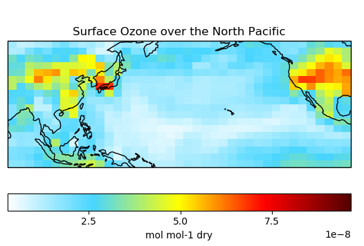
# Plot surface Ozone over the North Pacific
single_panel(
ds['SpeciesRst_O3'].isel(lev=0),
title='Surface Ozone over the North Pacific',
extent=[80, -90, -10, 60]
)
plt.show()
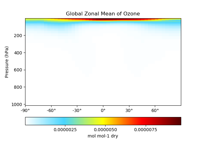
Zonal mean example:
# Plot global zonal mean of Ozone
single_panel(
    ds['SpeciesRst_O3'],
    plot_type='zonal_mean',
    title='Global Zonal Mean of Ozone'
)
plt.show()
Click here for an example single panel plotting script.
For detailed documentation, click on gcpy.plot.single_panel().
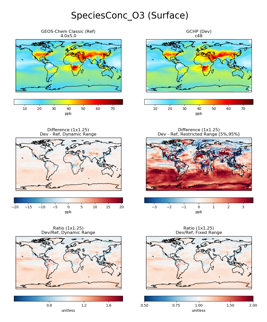
Six-panel comparison plots
Six-panel plots are used to compare results across two different model runs. Single level and zonal mean plotting options are both available. The two model runs do not need to be the same resolution or even the same grid type (GEOS-Chem Classic and GCHP output can be mixed at will).
Single level comparison:
import xarray as xr
import matplotlib.pyplot as plt
from gcpy.plot.compare_single_level import compare_single_level
from gcpy.plot.compare_zonal_mean import compare_zonal_mean

# Read data
gcc_ds = xr.open_dataset(
    'GEOSChem.SpeciesConc.20160701_0000z.nc4'
)
gchp_ds = xr.open_dataset(
    'GCHP.SpeciesConc.20160716_1200z.nc4'
)

# Plot comparison of surface ozone over the North Pacific
compare_single_level(
    gcc_ds,
    'GEOS-Chem Classic',
    gchp_ds,
    'GCHP',
    varlist=['SpeciesConc_O3'],
    extra_title_txt='Surface'
)
plt.show()
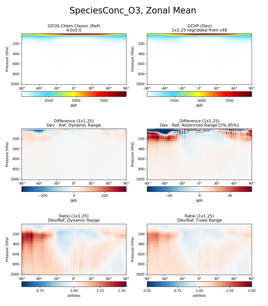
Zonal mean comparison:
# Plot comparison of global zonal mean ozone
compare_zonal_mean(
    gcc_ds,
    'GEOS-Chem Classic',
    gchp_ds,
    'GCHP',
    varlist=['SpeciesConc_O3']
)
plt.show()
Click here for an example six panel plotting
script. For complete documentation, click on
gcpy.plot.compare_single_level() and
gcpy.plot_compare_zonal_mean().
Comprehensive benchmark plotting
The GEOS-Chem Support Team uses comprehensive
plotting functions (see gcpy.benchmark.modules()) to generate
plots and tables from of diagnostic output of GEOS-Chem benchmark
simulations. Functions like
gcpy.benchmark.modules.make_benchmark_conc_plots generate plots
for every variable in a given collection
(e.g. SpeciesConc) at multiple vertical levels (surface,
500hPa, zonal mean) and divide plots into separate folders based on
category (e.g. Chlorine, Aerosols). For more information about the
benchmark plotting and tabling scripts, please see our
Benchmarking chapter.
Table creation
GCPy has several dedicated functions for tabling GEOS-Chem output data in text file format. These functions and their outputs are primarily used for model benchmarking purposes.
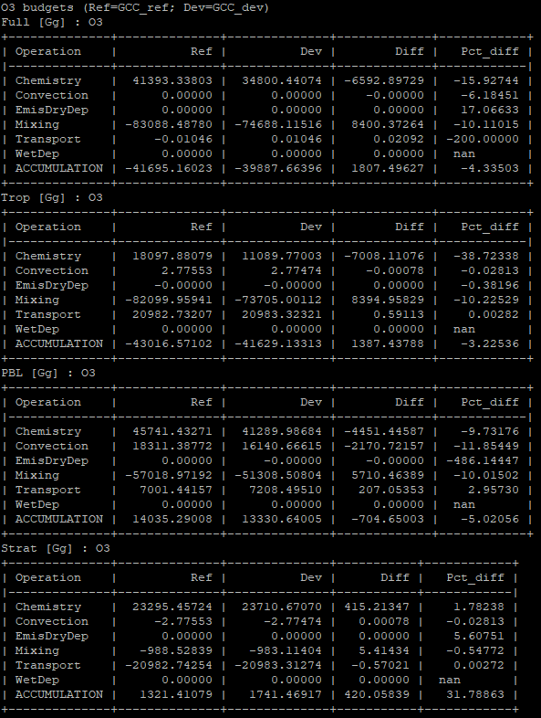
Budget tables
Currently, budget tables can be created for “operations” (table shows
change in mass after each category of model operation, as contained in
the GEOS-Chem Budget diagnostics) or in overall averages for
different aerosols or the Transport Tracers simulation.
Operations budget tables are created using the
gcpy.benchmark.modules.benchmark_funcs.make_benchmark_operations_budget()
function and appear as follows:
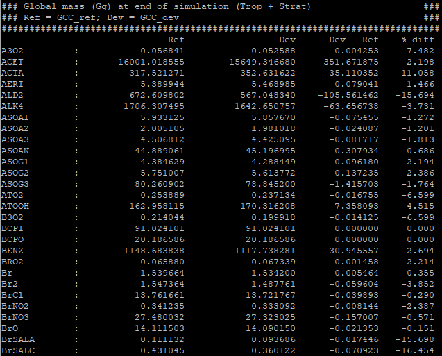
Mass tables
The
gcpy.benchmark.modules.benchmark_funcs.make_benchmark_mass_tables()
function uses species concentrations and info from meteorology files
to generate the total mass of species in certain segments of the
atmosphere (currently global or only the troposphere). An example
table is shown below:
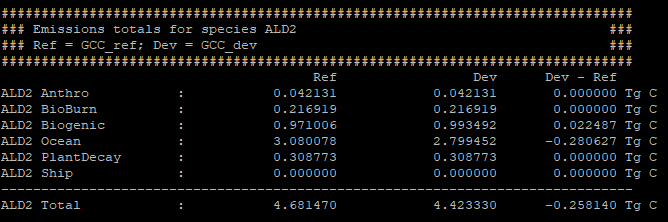
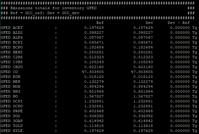
Emissions tables
The
gcpy.benchmark.modules.benchmark_funcs.make_benchmark_mass_tables()
function creates tables of total emissions categorized by species or by
inventory. Examples of both emissions table types are shown below:
Regridding
General regridding rules
GCPy supports regridding between all horizontal GEOS-Chem grid types, including latitude/longitude grids (the grid format of GEOS-Chem Classic), standard cubed-sphere (the standard grid format of GCHP), and stretched-grid (an optional grid format in GCHP). GCPy contains several horizontal regridding functions built off of xESMF. GCPy automatically handles most regridding needs when plotting GEOS-Chem data.
gcpy.file_regrid() allows you to regrid GEOS-Chem Classic and
GCHP files between different grid resolutions and can be called from
the command line or as a function.
gcpy.regrid_restart_file() allows you to regrid GCHP files
between between different grid resolutions and grid types
(standard and stretched cubed-sphere grids), and can be
called from the command line.
The 72-level and 47-level vertical grids are pre-defined in GCPy. Other vertical grids can also be defined if you provide the A and B coefficients of the hybrid vertical grid.
When plotting data of differing grid types or horizontal resolutions
using gcpy.plot.compare_single_level()
or gcpy.plot.compare_zonal_mean(), you
can specify a comparison resolution using the cmpres
argument. This resolution will be used for the difference panels in
each plot (the bottom four panels rather than the top two raw data
panels). If you do not specify a comparison resolution, GCPy will
automatically choose one.
For more extensive regridding information, visit the detailed regridding documentation.