Plotting

This page describes in depth the general plotting capabilities of GCPy, including possible argument values for every plotting function.

For information about GCPy functions that are specific to the GEOS-Chem benchmark workflow, please see our Benchmarking chapter.

Six-panel comparison plots

Functions gcpy.plot.compare_single_level() and gcpy.plot.compare_zonal_mean() generate six-panel plots comparing each variable between two datasets. These plots can either be saved to PDFs or generated sequentially for visualization in the Matplotlib GUI using matplotlib.pyplot.show(). Each plot uses data passed from a reference (Ref) dataset and a development (Dev) dataset. Both functions share significant structural overlap both in output appearance and code implementation.

You can import these routines into your code with these statements:

from gcpy.plot.compare_single_level import compare_single_level
from gcpy.plot.compare_zonal_mean import compare_zonal_mean

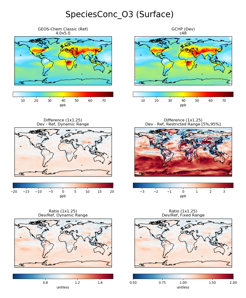
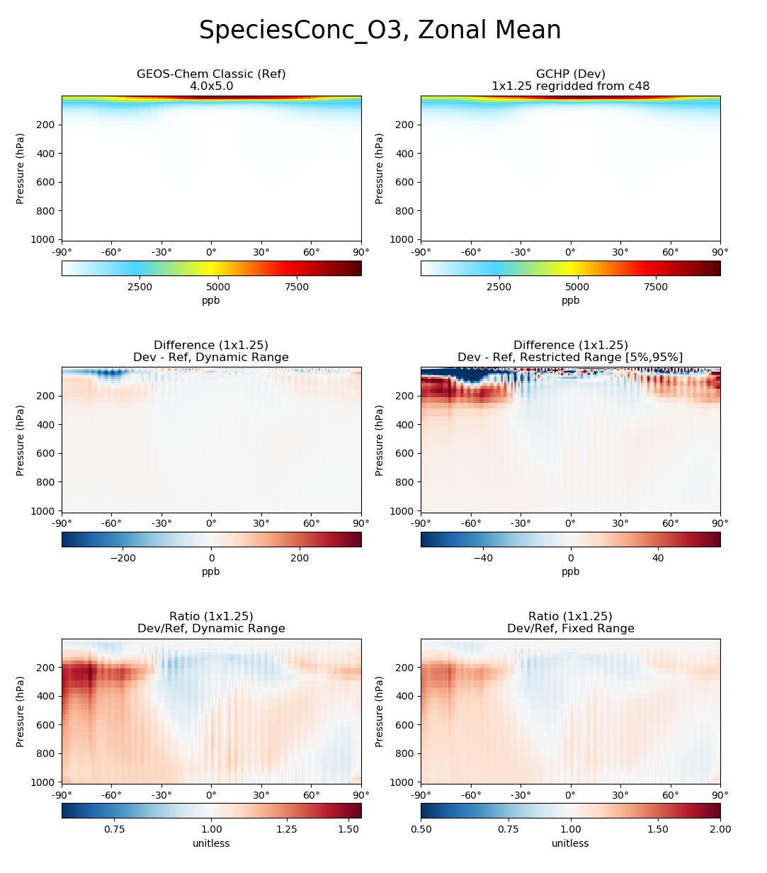
Each panel has a title describing the type of panel, a colorbar for the values plotted in that panel, and the units of the data plotted in that panel. The upper two panels of each plot show actual values from the Ref (left) and Dev (right) datasets for a given variable. The middle two panels show the difference (Dev - Ref) between the values in the Dev dataset and the values in the Ref dataset. The left middle panel uses a full dynamic color map, while the right middle panel caps the color map at the 5th and 95th percentiles. The bottom two panels show the ratio (Dev/Ref) between the values in the Dev dataset and the values in the Ref Dataset. The left bottom panel uses a full dynamic color map, while the right bottom panel caps the color map at 0.5 and 2.0.

Function compare_single_level

This function generates a comparison plot such as:

For a list of input parameters, click on this link: gcpy.plot.compare_single_level().

Function compare_zonal_mean

This function generates a comparison plot such as:

For a list of input parameters, click on this link: gcpy.plot.compare_single_level().

Shared structure

Both gcpy.plot.compare_single_level() and gcpy.plot.compare_zonal_mean() have four positional (required) arguments.

refdata <xarray.Dataset>

Dataset used as reference in comparison

refstr <str> | <list of str>

String description for reference data to be used in plots OR list containing [ref1str, ref2str] for diff-of-diffs plots

devdata : xarray.Dataset

Dataset used as development in comparison

devstr <str> | <list of str>

String description for development data to be used in plots OR list containing [dev1str, dev2str] for diff-of-diffs plots

refstr and devstr title the top two panels of each six panel plot.

Functions gcpy.plot.compare_single_level() and gcpy.plot.compare_zonal_mean() share many arguments. Some of these arguments are plotting options that change the format of the plots:

For example, you may wish to convert units to \(\mu\)g/m³ when generating comparison plots of aerosol species. Activate this option by setting the keyword argument convert_to_ugm3=True.

Other arguments are necessary to achieve a correct plot depending on the format of refdata and devdata and require you to know certain traits of your input data. For example, you must specify if one of the datasets should be flipped vertically if Z coordinates in that dataset do not denote decreasing pressure as Z index increases, otherwise the vertical coordinates between your two datasets may be misaligned and result in an undesired plotting outcome. This may be done with by setting the boolean options flip_ref=True and/or flip_dev=True.

The n_job argument governs the parallel plotting settings of gcpy.plot.compare_single_level() and gcpy.plot.compare_zonal_mean(). GCPy uses the JobLib library to create plots in parallel. Due to limitations with matplotlib, this parallelization creates plots (pages) in parallel rather than individual panels on a single page. Parallel plot creation is not enabled when you do not save to a PDF. The default value of n_job=-1 allows the function call to automatically scale up to, at most, the number of cores available on your system.

Note

On systems with higher (12+) core counts, the maximum number of cores is not typically reached because of the process handling mechanics of JobLib. However, on lower-end systems with lower core counts or less available memory, it is advantageous to use n_job to limit the max number of processes.

Due to how Python handles memory management on Linux systems, using more cores may result in memory not returned to the system after the plots are created. Requesting fewer cores with n_job may help to avoid this situation.

Example script

Here is a basic script that calls both gcpy.plot.compare_zonal_mean() and gcpy.plot.compare_single_level():

#!/usr/bin/env python

import xarray as xr
import matplotlib.pyplot as plt
from gcpy.plot.compare_single_level import compare_single_level
from gcpy.plot.compare_zonal_mean import compare_zonal_mean

file1 = '/path/to/ref'
file2 = '/path/to/dev'
ds1 = xr.open_dataset(file1)
ds2 = xr.open_dataset(file2)
compare_zonal_mean(ds1, 'Ref run', ds2, 'Dev run')
plt.show()
compare_single_level(ds1, 'Ref run', ds2, 'Dev run')
plt.show()

Single panel plots

Function gcpy.plot.single_panel() is used to create plots containing only one panel of GEOS-Chem data. This function is used within gcpy.plot.compare_single_level() and gcpy.plot.compare_zonal_mean() to generate each panel plot. It can also be called directly on its own to quickly plot GEOS-Chem data in zonal mean or single level format.

The gcpy.plot.single_panel() function expects data with a 1-length (or non-existent) T (time) dimension, as well as a 1-length or non-existent Z (vertical level) dimension. It also contains a few amenities to help with plotting GEOS-Chem data, including automatic grid detection for lat/lon or standard cubed-sphere xarray.DataArray()-s. You can also pass NumPy arrays to plot, though you’ll need to manually pass grid info in this case (with the gridtype, pedge, and pedge_ind keyword arguments).

The sample script shown below shows how you can data at a single level and timestep from an xarray.DataArray() object.

#!/usr/bin/env python

import xarray as xr
import matplotlib.pyplot as plt
from gcpy.plot.single_panel import single_panel

# Read data from a file into an xr.Dataset object
dset = xr.open_dataset('GEOSChem.SpeciesConc.20160701_0000z.nc4')

# Extract ozone (v/v) from the xr.Dataset object,
# for time=0 (aka first timestep) and lev=0 (aka surface)
sfc_o3 = dset['SpeciesConcVV_O3'].isel(time=0).isel(lev=0)

# Plot the data!
single_panel(sfc_o3)
plt.show()